
The Topic Correlations view helps you discover which themes in your data tend to appear together, and the Correlation Explanation shows why they’re connected.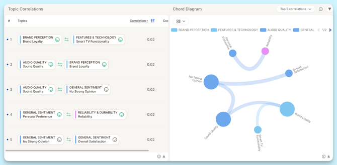
What It Shows
Caplena automatically detects relationships between topics that are frequently mentioned in the same responses.
Each row in the table represents a pair of correlated topics, showing how strongly they are linked.
The correlation score (r) tells you the strength of the relationship:
-
Higher values mean the topics co-occur more often.
Example:
Audio Quality ↔ Visual Quality (r = 0.53)
→ Respondents who mention sound quality also often talk about picture quality.
This allows you to see not just individual topics, but how they interact and shape overall perception.
Switch Between Views
On the right-hand side, you can explore your correlations in two different views:
Chord Diagram
A visual map showing how your topics connect.
-
Each bubble represents a topic.
-
Lines show connections between topics — the thicker the line, the stronger the correlation.
-
Bubble size reflects how frequently a topic appears in your dataset.
Hover over a topic to highlight its links or click to explore specific relationships.
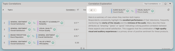
Correlation Explanation
When you switch to this view, Caplena’s AI provides a written summary explaining the connection between the selected topics.
How the Correlation Metric Is Calculated
The correlation score you see in Caplena is based on the Kulczyński measure (pronounced Kool-chin-ski 😉).
This score ranges from 0 to 1 and shows how likely two topics are to appear together.
-
A value close to 1 means the topics are strongly related.
-
A value close to 0 means they rarely appear together.
Unlike simpler methods, this measure also takes into account how often each topic appears, so it works well even if one topic is mentioned far more often than the other.
The idea behind it
You can think of it like this:
The Kulczyński score looks at “If I see Topic A, how often do I also see Topic B?”, and vice versa, then takes the average of both.
That’s why it’s great for spotting balanced, meaningful relationships rather than random overlaps
Formula:
0.5∗(A/(A+B)+A/(A+C))
Where:
-
A = number of responses mentioning both topics
-
B = number of responses mentioning only topic 1
-
C = number of responses mentioning only topic 2
We want to calculate the Kulczinsky value between Design and Product.
- Design and Product have been mentioned together 55 times, so A =100
- Design has been mentioned 20 times (without Product), so B = 20
- Product has been mentioned 80 times (without Design), so C = 80
The Kulczinsky value would be calculated the following way :
0.5 * ( 100/120 + 100/180) = 0.7
Below are a few examples showing how the Kulczyński value is calculated depending on how often two topics appear together.
Example 1: Rare co-occurrence
If Topic A occurs in 100 rows and Topic B in only 1 row (which also contains Topic A), the calculation is:
Kulczyński = 0.5 * (1 / 100 + 1 / 1) = 0.505
Even though Topic B appears only once, it always co-occurs with Topic A, resulting in a moderate similarity score.
Example 2: Moderate co-occurrence
If Topic A occurs in 100 rows and Topic B in 100 rows, and both appear together in 50 rows:
Kulczyński = 0.5 * (50 / 100 + 50 / 100) = 0.50
Both topics appear frequently and together in half of the cases, giving a moderate relationship score.
Example 3: Strong co-occurrence
If Topic A occurs in 50 rows and Topic B in 100 rows, and they appear together in 50 rows:
Kulczyński = 0.5 * (50 / 50 + 50 / 100) = 0.75
Topic A always appears with Topic B, a strong connection between the two.
| Topic A Mentions | Topic B Mentions | Both Together | Kulczyński | What It Means |
|---|---|---|---|---|
| 100 | 100 | 50 | 0.50 | They appear together half of the time, moderately related. |
| 100 | 1 | 1 | 0.505 | Topic B is rare, but every time it appears, it’s with A, still a noticeable link. |
| 50 | 100 | 50 | 0.75 | Every time A appears, it’s with B, a strong connection. |